Dissipative XXZ Chain

A many-body spin system becomes an open quantum system when it exchanges energy or information with an environment. A standard example is an interacting XXZ chain subject to local spontaneous emission.

We consider the Hamiltonian

\[H = \sum_{i<j} J_{ij} \left[ J_{xy} \left( \sigma_i^+ \sigma_j^- + \sigma_i^- \sigma_j^+ \right) + J_z \sigma_i^z \sigma_j^z \right],\]

with nearest-neighbor couplings and local collapse operators

\[L_i = \sqrt{\gamma}\,\sigma_i^-.\]

The density matrix obeys the Lindblad master equation

\[\frac{d\rho}{dt} = -i[H,\rho] + \sum_i \left( L_i \rho L_i^\dagger - \frac{1}{2} \left\{ L_i^\dagger L_i,\rho \right\} \right).\]

Starting from a Néel state, coherent XXZ interactions compete with irreversible spin relaxation.

Model

using OpenSpinDynamics
using SparseArrays
using CairoMakie

N = 4
γ = 0.3

coupling = NearestNeighborCoupling(
    0.0,
    N,
)

model = SpinModel(
    N;
    Jxy=1.0,
    Jz=0.5,
    coupling=coupling,
)

ops = spin_operators(N)

Initial state

We initialize the chain in a Néel product state,

\[|\psi_0\rangle = |\uparrow\downarrow\uparrow\downarrow\rangle,\]

and convert it to a density matrix.

ψ0 = neel_state(
    N;
    direction=:z,
)

ρ0 = sparse(ψ0 * ψ0')

Local decay

Each spin is coupled independently to a zero-temperature environment through a lowering operator.

lindblad_ops = [
    sqrt(γ) * ops.minus[i]
    for i in 1:N
]

Observables

We monitor two quantities.

The average longitudinal magnetization is

\[M_z = \frac{1}{N} \sum_{i=1}^{N} \sigma_i^z,\]

while the staggered magnetization is

\[M_s = \frac{1}{N} \sum_{i=1}^{N} (-1)^{i-1}\sigma_i^z.\]

Mz = sum(
    ops.z[i]
    for i in 1:N
) / N

Mstag = sum(
    (-1)^(i - 1) * ops.z[i]
    for i in 1:N
) / N

times = collect(
    range(0.0, 4.0; length=121)
)

For the initial Néel state, the uniform magnetization is zero while the staggered magnetization is one.

initial_Mz = real(ψ0' * Mz * ψ0)
initial_Mstag = real(ψ0' * Mstag * ψ0)

(initial_Mz, initial_Mstag)

(0.0, 1.0)

Lindblad evolution

For this small chain we use the exponential Lindblad backend.

result = evolve(
    model,
    ρ0,
    times,
    [Mz, Mstag];
    method=:expm,
    lindblad_ops=lindblad_ops,
)

The first column contains $\langle M_z\rangle$ and the second contains $\langle M_s\rangle$.

Magnetization dynamics

fig = Figure(size=(720, 430))

ax = Axis(
    fig[1, 1];
    xlabel="Time",
    ylabel="Magnetization",
    title="Dissipative XXZ chain with local decay",
)

lines!(
    ax,
    times,
    result[:, 1];
    label="Average magnetization",
    linewidth=2,
)

lines!(
    ax,
    times,
    result[:, 2];
    label="Staggered magnetization",
    linewidth=2,
)

axislegend(ax)

fig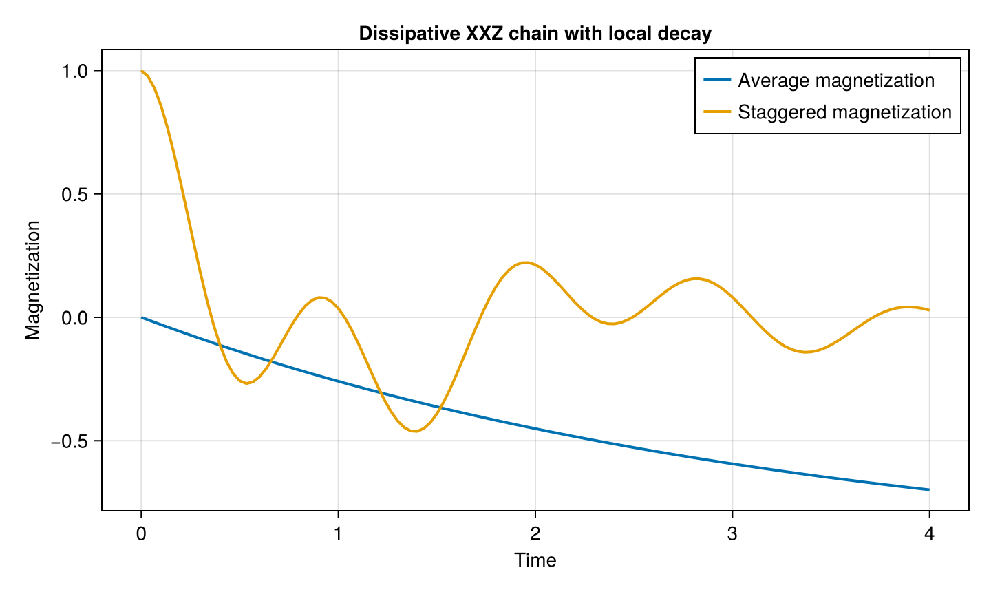

The staggered order decreases as the interacting system evolves away from the initial Néel state. At the same time, spontaneous emission drives the spins toward the down-polarized state, causing the average longitudinal magnetization to become increasingly negative.

This example combines coherent many-body XXZ dynamics with local Markovian dissipation using the same high-level evolve interface.